Let’s admit, most of us common Windows users dread numbers and spreadsheets. But fear not! There are several useful tips for entering formulas in spreadsheets and getting the most out of MS Excel.
These tips are easy to apply even for those who rarely use such programs. Plus, having a clear understanding of MS Excel is essential to get the correct results from your data. Join us for a list of 7 MS Excel formula tips and tricks to help you get started!
Also learn how to insert check mark in MS Excel
1. The simplest approach is to focus on the details as you work. Ensure that you type the formula in the right cell. You can also select multiple cells and use the "Copy here as values only" option. This method will copy the values in the cells you selected without using default cell references. You can apply the method to a single cell or a range of consecutive cells. If you want to apply a formula to multiple cells in one sheet, hold down Ctrl while clicking the selection button.
- Another helpful tip is to convert a selected part of the excel sheet into a table. If you have specific rows and columns of data that are hard to work it, making a table can help sort and see it better. This can increase your productivity.
a. First, select your data.
b. Then press Ctrl+T. confirm the data selected and click OK.
c. Now you can easily view the numbers as a formatted table.
3. You can switch rows to columns or columns to rows in Excel. You can do this with a function called “Transpose”. To transpose data, execute the following steps:
a. Select the data range you want to transpose e.g. A1:D1. Right-click, and then click Copy.
b. Select the destination cell, right-click, and select Paste Special.
c. Check Transpose. Click OK.
4. If you have lots of data, there is a way to narrow down the cells you want.
a. First, select a single cell to search for the entire sheet, or a range of cells to search for a limited portion of it. The F5 (you may use the fn key on some keyboards), as well as the Ctrl+G keyboard shortcut, open the Go to the dialog box.
b. Click on the "Special" option there, and it opens a pop-up with many options to select.
If you select the Formulas option and click OK, this highlights the portions of the spreadsheet where you used the formulas.
5. Numerous users use the SUM () function in MS-Excel, but you do not have to type this command again and again. Most users use this function to add numbers. However, you can also make it easier by using the AutoSum keyboard shortcut.
a. Select the data in a column and press Alt + =. This function will automatically calculate the range of values that need to be summed.
If you have more than one parameter in your formula, you should try breaking them into different columns.
6. A common way to select all the data in a single spreadsheet is to press Ctrl + A. But few know that you can select all sheet content by clicking the small triangle at the left corner as shown in the screenshot. This will select all the data in a sheet, except for the graphs.
7. In the rows and columns, some default data will be blank, for various reasons. To maintain accuracy and to clean up unnecessary blank cells. The quickest way to delete the blank cells is to filter out all blank cells and delete them with one click. To do this:
a. Choose the column you want to filter, then go to the Data tab and click ‘Filter’.
b. Return to the selected data. A drop-down arrow will appear on the top of the column. Click the drop-down arrow. Under the ‘Search’ section, you will find various checkboxes. First, uncheck “Select All”.
Learn how to create drop-down list in MS Word
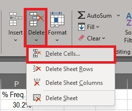
c. In the end, there is a checkbox named ‘Blanks’. Check this box and click OK.
d. All blank cells will show instantly. Go to the Home tab, and click Delete > Delete Cells. This will delete all the blank cells in your data.
I hope you will find these tips useful. If you have any suggestions, you can give your comments below.